Multisite adaption algorithm based on low-rank representaion: Criticizing a paper and developing my own algorithm, which is also full of flaws.

You may wanna read my note on low-rank representaion and the paper on multi-site adaption based on low-rank representation.

Part 1: Problems about this paper

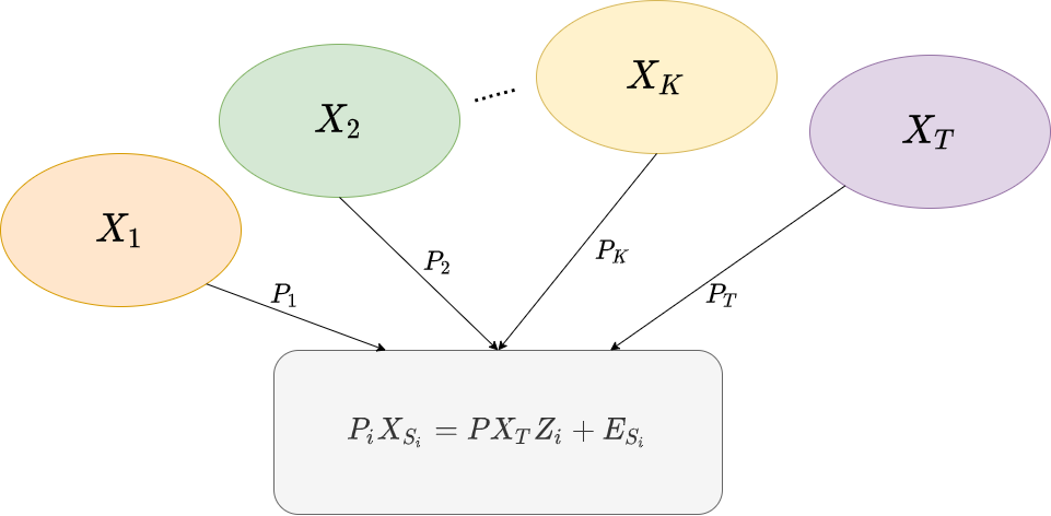
In the paper, the basic set up is: data come from $T$ different sites, each site may have some systematic bias which make data from different sites somewhat "heterogeneous". Then from these $T$ sites, choose one as "Target Site" $S_T$, assume there is a projection matrix $P$ which maps data from $S_T$ to the common latent space. Then for each of other sites $S_i$, which are called a "Source Site", there is a projection matrix $P_i$, obtained by $P_i = P + E_{P_i}$, which maps data from $S_i$ to the latent space. Then use the mapped data from the target site to linearly represent the mapped data from source sites, that is $P_iX_{S_i} = PX_TZ_i + E_{S_i}$, where $X_{S_i}$ is the data from source site $S_i$ and $X_T$ is the data from target site $S_T$.The setup is illustrate by the picture below.

It's assumed that the latent space is low-rank, then the following optimization problem is given

This problem can be solved by solving the equivalent problem

Then the paper solve this problem with Augmented Lagrangian Multiplier. First, form the augmented lagrangian multiplier as if the constraint $PP^T=I$ does not exist.

Then the optimization algorithm is given

initialize all variables
while not convergence{
    Fix other variables, minimize A_c over J
    Fix other variables, minimize A_c over F_i 
    Fix other variables, minimize A_c over E_{S_i}
    Fix other variables, minimize A_c over E_{P_i}
    Fix other variables, minimize A_c over F_i
    Fix other variables, minimize A_c over Z_i
    Fix other variables, minimize A_c over P_i
    Fix other variables, minimize A_c over P
    Update dual variable Y_{1,i} += Z_i - F_i
    Update dual variable Y_{2,i} += Z_i - F_i
    Update dual variable Y_{3,i} += Z_i - F_i
    Update dual variable Y_1 += Z_i - F_i
    
    P = Orth(P) to satisfy PP^T = I
}

I found 3 fatal mistakes in this article.

1. About the objective

In this article, one term in the the objective of the optimization problem is $||P||_*$, which is the sum of singular values of $P$. But when the equality constraint $PP^T=I$ is satisfied, we can perform singular value decomposition on $P$, we will get

Multiplie both sides by $U$, we get $U \Sigma^2=U$ Since $\Sigma$ is a diagonal matrix, the only solution is that $\Sigma=I$. If so, $P = U \Sigma V^T$ has nuclear norm $n$, then the term $||P||_*$ is determined by $PP^T=I$. So the term $||P||_*$ in the objective is redundant.

2. About the optimization problem

The optimization algorithm given by this article is not quite justified.

They constructed the Augmented Lagrangian Multiplier as if the equality constraint $PP^T=I$, which is a quadratic constraint, does not exist. After each iteration where the primal and dual variables are minimized over, the constraint $PP^T=I$ is satisfied by "bruteforcely" orthogonalizing$P$, this step changes $P$, thus $P$ does not minimizes the lagrangian when other variables are fixed, so the convergence of augmented lagrangian multiplier does not hold any more.

If this algorithm does converge with some magic going on underneath, at least they can give some proof or say something like "we cannot prove the convergence but it does converge everytime in the experiment".

3. About the convexity

As I quote from the paper, "the optimization of Eq.(5) is convex and can be solved by iteratively updating each variable separately".

Even if we do not consider this equality constraint $PP^T=I$, which is not included when forming augmented lagrangian multiplier, the equality constraint $P_i X_{S_i} = P X_T Z_i + E_{S_i}$, which is a quadratic equality constraint because of the appearance of variables $P$ and $Z_i$ in the same term, makes the problem nonconvex.

Thus the optimization problem is in no sense convex due to a quadratic equality constraint. There are some convergence proof for augmented lagrangian multiplier on nonconvex problems, but the statement "the optimization of Eq.(5) is convex" is definitely wrong.

---

So, there are 2 possibilities

1. I do not fully understand this paper, if you find where I was wrong, please email diqiudaozhezhuan@gmail.com, it really bothers me.
2. This article is full of flaws.

When thinking through this article, I came up with my own idea, which turns out to be also a piece of garbage. But I still wanna write it down.

Part 2: My own idea.

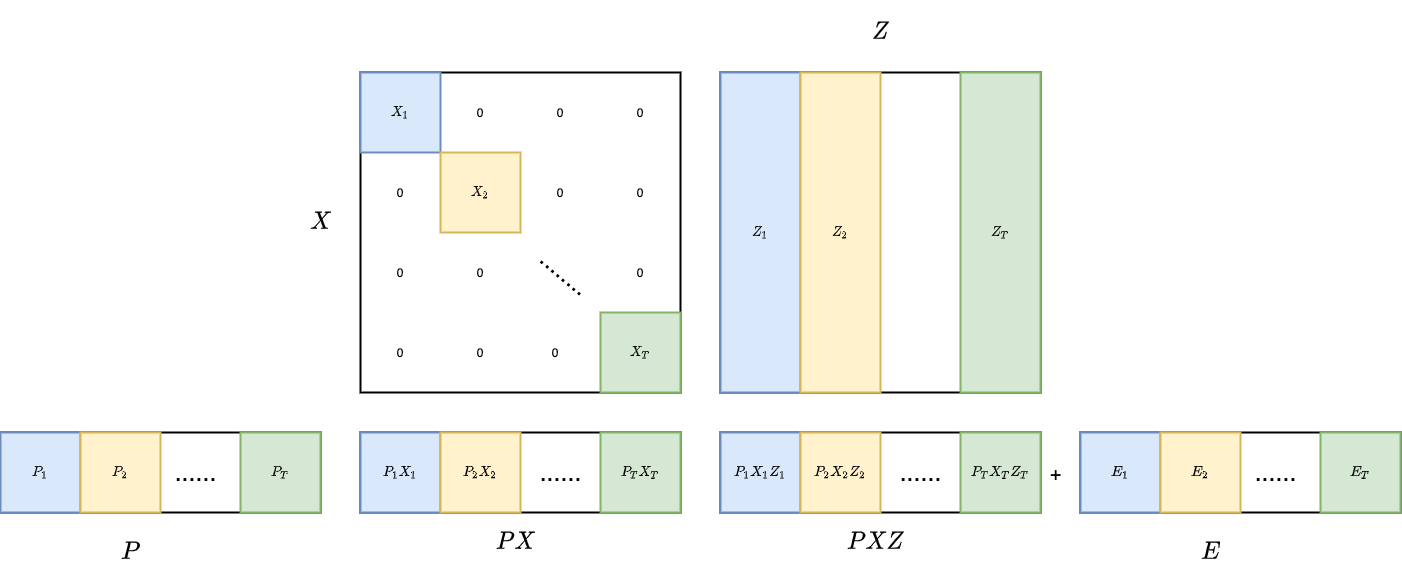
Actually, my idea is very simple. Suppose datas from differents sites came from a common space, for each site $S_i$, there is a projection matrix $P_i$ which project the data to a common space, then perform low-rank representation in the common space. We can arrange $X_i$'s into a block-diagonal matrix $X$ and horizontally stack $P_i$'s in to a matrix $P$. And the optimization problem can be written as

This is identical to the basic low-rank representation except that here we perform low-rank representation with $PX$. The structure of the matrix multiplication is shown in the picture below.

However, this optimization has a trivial solution $P=0, Z=0, E=0$. This trivial solution exists because that when mapping datas to a common space, we through all informations in $X$ by setting $P=0$, thus the common space is surely low-rank. Thus, we want to project $X$ into the common space and keep some information in $X$ in the meantime. Consider the following optimization problem

The term $||P_i - I||_*$ in objective is quite heuristic, that is, put it other way, not fully justified. The motivation is, if $||P_i - I||_*$ is small, then the sigular values of $P_i - I$ tends to 0, then singular values of $P_i$ tends to 1, thus we avoid the situation where $P_i$ throws all information in $X$.

This problem is nonconvex due to the quadratic equality constraint $PX=PXZ+E$,but we can still use augmented lagragian multiplier to get to a local minimum.

To solve the optimization problem, we can solve the equivalent problem

First, we build the augmented lagrangian multiplier

We can alternatively minimize the lagrangian over each variable.

1. minimize over $J$

This gives the optimization problem

The close-form solution is given by singular value shrinkage

2. minimize over $Q_i$

This gives the optimization problem

The close-form solution is given by singular value shrinkage

3. minimize over $P$

This gives the optimization problem

This problem can be dissect into several optimization problems

where $F_i$ is the ith row block of $I-Z$.

The close-form solution is given by

4. minimize over $Z$

This gives the optimization problem

The close-form solution is given by

Implementation details: In (3) and (4),the "diagonal-plus-lowrank" structure is crying out, make sure that you exploit the sparsity pattern by using block elimination to solve the linear system

5. minimize over $E$

This gives the optimization problem

This problem can be dissected into several problems

where $F_i$ is the ith column block of $I_Z$, $Y_{1,i}$ is the ith column of the dual variable $Y_1$.

This problem can be formulated as below

which can be solved efficiently with primal-dual interior point method. For the detail, please refer to and appendix.

We can alternatingly optimize over each variable and update the dual variable accordingly in each iteration of augmented lagrangian multiplier.

---

This method also have some problems.

1. About the objective

The term $||P_i-I||_*$ make the singular values of $P_i$ tend to 1. However, we have no idea that the "right" solution for $P$ have all 1 singular values. We can only prevent $P$ from throwing away all information in$X$.

2. About the convexity

Due to the equality constraint $PX=PXZ + E$, the problem is nonconvex. Though we can get a local minimum by using the augmented lagrangian multiplier and achieve a "fairly good" solution by running multiple trials with different initial points, it's not as elegant as a convex problem.

3. About the complexity

In each iteration, assuming there are $K$ sites and each data has dimension $n$, we'll need to solve $K$ $n \times n$ SVDs when calculating $(2)$, each of which has complexity $O(n^3)$. When the data is high-dimension, the problem becomes intractable quickly.

Part 3: Results of my own idea.

Following is the result on Yale face dataset when I set $\alpha=0.5$ and $\beta=0.05$.

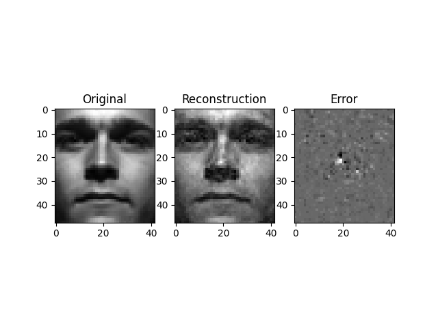
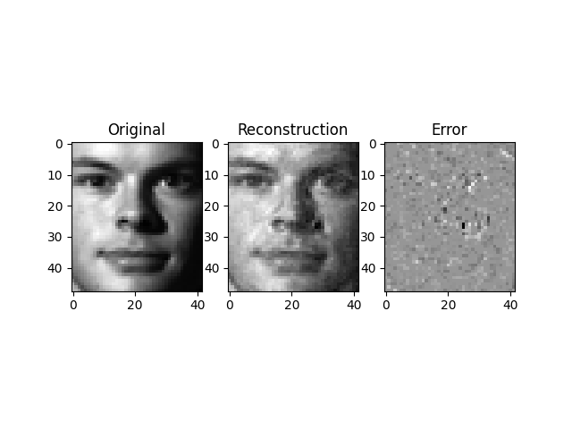
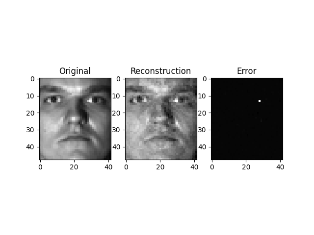
These images have lower quality after low-rank representaion, but remember that the purpose of low-rank representation if to map data into a common space. In these results, the shade at the eye is eliminated in the first image and the shade near the nose is eliminated in the second image, making those two images pretty "homogeneous".

Only one experiment was done since solving the optimization problem is pretty time-consuming. I think the result can be better if proper $\alpha$ and $\beta$ is chosen.

4. Appendix : Solving one-norm-plus-frobenius-norm-square

Consider the optimization problem

This can be reformulated into an equivalent problem

which is differentiable.

Write this into a standard form

with a change of notation, we can write the problem as

Form the Lagrangian

the modified KKT condition for the log barrier is

The residual is given by

Then form the KKT system

where $rd$ and $rc$ stand for dual residual and centrality residual, respectively. Then solve the KKT system by block elimination

For more detail about primal-dual interior point method, refer to my note.

Implementation details: Notice the structure of matrices and make sure you exploit the sparsity in solving the KKT system.