Decision Tree

Example

To build an intuition what a decision tree is, let's first see an example.

Suppose some vampires are mixed in us on campus, and we want to find them out.

Here're some samples and we want to come up with some rules that someone maybe a vampire.(? means unknown)

Vampire	Shadow	Garlic	Complexion	Accent
No	?	Yes	Pale	None
No	Yes	Yes	Ruddy	None
Yes	?	No	Ruddy	None
Yes	No	No	Average	Heavy
Yes	?	No	Average	Odd
No	Yes	No	Pale	Heavy
No	Yes	No	Average	Heavy
No	?	Yes	Ruddy	Odd

And we may build a decision tree like this:

After many test we still cannot decide whether he's a vampire, it seems that this decision tree didn't do well.

We can see that decision tree is just a fancy saying of a set of if-then rules.

Let find out how we can build a better decision tree.

Decision Tree Learning

Decision Tree Learning, given a training dataset of size:

D = \{ (x_1,y_1),...,(x_m,y_m) \}

x^{(i)} = (x_1^{(i)}, x_2^{(i)},...,x_n^{(i)})^T

m is the size of training data, and n is the feature dimension.

Essentially, decision tree learning is to conclude a set of dicision rule.

There can be many decision trees that not conflict with the training dataset, one of them, or even none of them.

So what we need is a decision tree that confilct least with training dataset, and do well in generalization.

From another perspective, decision tree learning is to simulate a condition probability distribution according to training dataset. The chosen condition probability distribution should not only fit the training dataset well, but also perform good prediction on unknown data.

Feature Selection

When we build a decision tree, we always want to more from one single given feature. Or more perfessionally, more infomation gain.

(If you're not familiar with information gain, you may want to check this note first.)

Remeber our vampire dicision tree didn't do well, may be it's because feature selection is not so reasonable??

Let's try to improve it with infomation gain theory.

First, review our samples.

Vampire	Shadow	Garlic	Complexion	Accent
No	?	Yes	Pale	None
No	Yes	Yes	Ruddy	None
Yes	?	No	Ruddy	None
Yes	No	No	Average	Heavy
Yes	?	No	Average	Odd
No	Yes	No	Pale	Heavy
No	Yes	No	Average	Heavy
No	?	Yes	Ruddy	Odd

What should be the first decision, aka, first if-then rule?

Let's test them all !!

First, the entropy of original dataset is

-\frac{3}{7}*log(-\frac{3}{7}) -\frac{3}{7}*log(-\frac{3}{7}) ≈ 0.98

Conditional Entropy

(Shadow test)

First, if we choose shadow as the first if-then rule.

The original samples are divided into 3 groups.

The entropy is (2-base):

Group1: $-\frac{1}{2} * log(\frac{1}{2}) -\frac{1}{2} * log(\frac{1}{2}) = 1$

Group2: $-1*log(1) = 0$

Group3: $-1*log(1) = 0$

According to the definition of conditional entropy: $H(Y|X) = \sum_{i=1}^np_i H(Y|X=x_i)$

Conditional entropy given shadow test is

1*\frac{4}{8} + 0*\frac{3}{8} * 0*\frac{1}{8} = 0.5

(Garlic test)

( -\frac{3}{5} * log(\frac{3}{5}) - -\frac{2}{5} * log(\frac{2}{5}) )*\frac{5}{8} ≈ 0.9 * \frac{5}{8} ≈ 0.6

(Complexion test)

( -\frac{2}{3} * log(\frac{2}{3}) - -\frac{1}{3} * log(\frac{1}{3}) )*\frac{3}{8}*2 ≈ 0.7

(Accent test)

( -\frac{2}{3} * log(\frac{2}{3}) - -\frac{1}{3} * log(\frac{1}{3}) )*\frac{3}{8}*2 ~ + ( -\frac{1}{2} * log(\frac{1}{2}) - -\frac{1}{2} * log(\frac{1}{2}) )*\frac{2}{8} ≈ 0.95

(You're encouraged to verify these equations by yourself !!)

Information Gain

Shadow test: $0.98-0.5 = 0.48$

Garlic test: $0.98-0.6 = 0.38$

Complexion test: $0.98-0.6 = 0.38$

Accent test: $0.98-0.95 = 0.03$

The shadow test has the greatest information gain, in other word, we get the most knowledge from shadow test, so we may want to choose shadow test as the first if-then rule of our decision tree.

And the decision tree now looks like this

We can see that in group #2 and group #3, there're no mix-up. And our training example becomes like this, leaving only samples in group #1.

Vampire	Shadow	Garlic	Complexion	Accent
No	?	Yes	Pale	None
Yes	?	No	Ruddy	None
Yes	?	No	Average	Odd
No	?	Yes	Ruddy	Odd

Now let continue building our decision tree. We're left with garlic test, complexion test, and accent test.

Let's do the calculation once more. The entropy of left samples is:

-\frac{2}{4}*log(\frac{2}{4}) -\frac{2}{4}*log(\frac{2}{4}) = 1

If we do garlic test, it's like this

And the conditional entropy is

(-1*log(1)) * \frac{2}{4} * 2 = 0

The information gain is

1-1=0

It's the max information gain, you can verify by yourself, so we choose garlic test as the second if-then rule of out decision tree.

Now our decision tree looks like this

After 2 tests we can decide whether a man is vampire.

We always choose the test with max infomation gain as the next test we'll perform on dataset left by previous test.

Implementation Decision Tree

Now let's implement a decision tree in Python to help us pick out the vampire in us !!

Create a python file, DTree.py

First, import useful libraries:

import numpy as np
import operator

Our vampire training set, notice that for conveience I put the label to the last column

def getSillyDataSet():
    dataset = [
        ['?',    'Yes',  'Pale',     'None',    'No',],
        ['Yes',  'Yes',  'Ruddy',    'None',    'No',],
        ['?',    'No',   'Ruddy',    'None',    'Yes'],
        ['No',   'No',   'Average',  'Heavy',   'Yes'],
        ['?',    'No',   'Average',  'Odd',     'Yes'],
        ['Yes',  'No',   'Pale',     'Heavy',   'No'],
        ['Yes',  'No',   'Average',  'Heavy',   'No'],
        ['?',    'Yes',  'Ruddy',    'Odd',     'No']
    ]

    featureName = ['Shadow','Garlic','Complexion', 'Accent']

    return dataset, featureName

Function to calculate entropy

def entropy(dataSet):
    numEntries = len(dataSet)

    labelCount = {}
    for featureVec in dataSet:
        label = featureVec[-1]
        labelCount[label] = labelCount.get(label, 0) + 1

    __entropy = 0.0
    for key in labelCount:
        prob = float(labelCount[key]) / numEntries
        __entropy -= prob * np.log2(prob)

    return __entropy

Data spliting, choose subdataset according to specific feature

def splitDataSet(dataset, axis, value):
    retDataSet = []
    for featureVec in dataset:
        if featureVec[axis] == value:
            # delete a feature since that we have make a if-then decision on that feature
            reducedFeatureVec = featureVec[:axis]
            reducedFeatureVec.extend(featureVec[axis+1:])
            #reducedFeatureVec = featureVec[:axis].extend(featureVec[axis+1:])
            retDataSet.append(reducedFeatureVec)
    return retDataSet

Choose which feature to measure to build next if-then rule, based on information gain

def chooseFeatureToSplit(dataSet):
    numFeatures = len(dataSet[0]) - 1
    baseEntropy = entropy(dataSet)

    bestInfoGain = 0.0
    bestFeature = -1
    for i in range(numFeatures):
        featureList = [example[i] for example in dataSet]
        uniqueFeatureVals = set(featureList)
        newEntropy = 0.0

        for val in uniqueFeatureVals:
            subDataSet = splitDataSet(dataSet, i, val)
            prob = len(subDataSet) / float(len(dataSet))
            newEntropy += prob * entropy(subDataSet)

        infoGain = baseEntropy - newEntropy

        if infoGain > bestInfoGain:
            bestInfoGain = infoGain
            bestFeature = i

    return bestFeature

If we have gone through all features and still cannot decide which class the sample belongs to, we need to treat it as the majority class of such samples.

def majorityCount(classList):
    classCount = {}
    for vote in classList:
        classCount[vote] = classCount.get(vote, 0) + 1

    sortedClassCount = sorted(classCount.iteritems(), key=operator.itemgetter(1), reverse=True)
    return sortedClassCount[0][0]

Now it's the key logic to build decision tree. Remeber when we learn tree in data structure, the structure of tree is recursive, it's reasonable to build a decision tree recursively.

(case 1)

The base case is, after a if-then rule, one group has the same label, that's when we stop.

(case 2)

And when we've gone through every features, or say, every if-then rule, we still cannot decide which class it is, now we treat it like the majority of that group.

(case3)

Else, choose the best feature, and devide dataset into groups, then build tree on each group.

def createTree(dataSet, feature_names):
    classList = [example[-1] for example in dataSet]
    
    # case 1
    if classList.count(classList[0]) == len(classList):
        return classList[0]
    
    # case 2
    if len(dataSet[0]) == 1:
        return majorityCount(classList)
    
    # case 3
    bestFeature = chooseFeatureToSplit(dataSet)
    bestFeatureName = feature_names[bestFeature]
    myTree = {bestFeatureName:{}}
    
    # remove a feature indicates that we gone through this feature
    __feature_names = feature_names[:]
    del (feature_names[bestFeature])

    featureValues = [example[bestFeature] for example in dataSet]
    uniqueVals = set(featureValues)

     for val in uniqueVals:
        subset = splitDataSet(dataSet, bestFeature, val)
        myTree[bestFeatureName][val] = createTree(subset, __feature_names)
    return myTree

Let's run the decision-tree-building program on our vampire dataset.

data, features = getSillyDataSet()
print createTree(data, features)

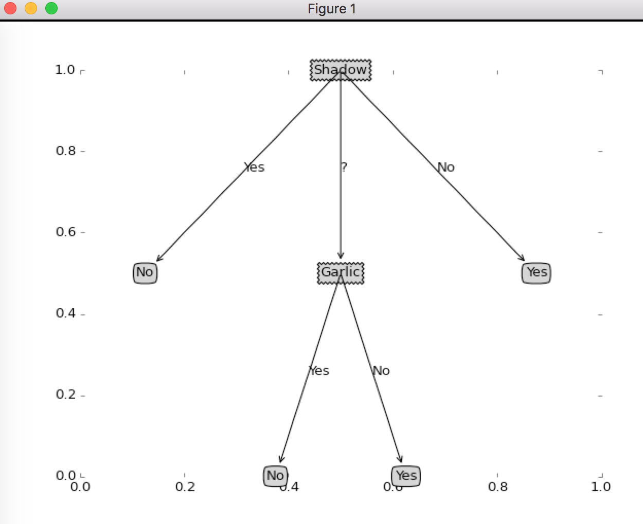
The output is

{'Shadow': {'Yes': 'No', '?': {'Garlic': {'Yes': 'No', 'No': 'Yes'}}, 'No': 'Yes'}}

It's visually excruciating, let's visualize it.

Create another python file DTreePlot.py.

import matplotlib.pyplot as plt

decisionNode = dict(boxstyle='sawtooth', fc='0.8')
leafNode = dict(boxstyle='round4', fc='0.8')
arrow_args = dict(arrowstyle='<-')



def plotNode(nodeText, centerPt, parentPt, nodeType):
    createPlot.ax1.annotate(nodeText, xy=parentPt, xycoords='axes fraction', xytext=centerPt,
                            textcoords='axes fraction', va='center', ha='center', bbox=nodeType, arrowprops=arrow_args)

def plotMidText(centerPt, parentPt, textString):
    xMid = (parentPt[0]-centerPt[0])/2.0 + centerPt[0]
    yMid = (parentPt[1]-centerPt[1])/2.0 + centerPt[1]
    createPlot.ax1.text(xMid, yMid, textString)


def plotTree(tree, parentPt, nodeText):
    numLeaf = getNumLeaf(tree)
    depth = getTreeDepth(tree)

    firstStr = tree.keys()[0]
    centerPt = (plotTree.xOff + (1.0 + float(numLeaf))/2.0/plotTree.totalW, plotTree.yOff)
    plotMidText(centerPt, parentPt, nodeText)
    plotNode(firstStr, centerPt, parentPt, decisionNode)
    secondDict = tree[firstStr]

    plotTree.yOff = plotTree.yOff - 1.0/plotTree.totalD

    for key in secondDict.keys():
        if type(secondDict[key]).__name__ == 'dict':
            plotTree(secondDict[key], centerPt, str(key))
        else:
            plotTree.xOff = plotTree.xOff + 1.0/plotTree.totalW
            plotNode(secondDict[key], (plotTree.xOff, plotTree.yOff), centerPt, leafNode)
            plotMidText((plotTree.xOff, plotTree.yOff), centerPt, str(key))
    plotTree.yOff = plotTree.yOff + 1.0/plotTree.totalD



def createPlot(tree):
    fig = plt.figure(1, facecolor='white')
    fig.clf()
    axprops = dict(xticks=[], yticks=[])
    createPlot.ax1 = plt.subplot(111,frameon=False)

    plotTree.totalW = float(getNumLeaf(tree))
    plotTree.totalD = float(getTreeDepth(tree))
    plotTree.xOff = -0.5/plotTree.totalW
    plotTree.yOff = 1.0
    plotTree(tree, (0.5,1.0),'')
    plt.show()


def getNumLeaf(tree):
    all_leaf = 0
    firstStr = tree.keys()[0]
    secondDict = tree[firstStr]

    for key in secondDict.keys():
        if type(secondDict[key]).__name__ == 'dict':
            all_leaf += getNumLeaf(secondDict[key])
        else:
            all_leaf += 1

    return all_leaf

def getTreeDepth(tree):
    maxDepth = 0
    firstStr = tree.keys()[0]   # dict for this test

    secondDict = tree[firstStr] # dict for groups of this test

    for key in secondDict.keys():
        if type(secondDict[key]).__name__ == 'dict':
            this_depth = getTreeDepth(secondDict[key]) + 1
        else:
            this_depth = 1
        if this_depth > maxDepth:
            maxDepth = this_depth
    return maxDepth

And in DTree.py

import DTreePlot

data, feature = getSillyDataSet()
tree = createTree(data, feature)
DTreePlot.createPlot(tree)

Our decision tree looks like this

Now, let's try to actually make a prediction on a decision tree.

In DTree.py

def classify(tree, features, sample):
    firstStr = tree.keys()[0]
    secondDict = tree[firstStr]
    
    # which feature the decision tree is using
    featureIdx = features.index(firstStr)

    for key in secondDict.keys():
        if sample[featureIdx] == key:
            
            # if further judgment is required
            if type(secondDict[key]).__name__ == 'dict':
                classLabel = classify(secondDict[key], features, sample)
            else:
                classLabel = secondDict[key]
    return classLabel

The order of if-then rules of decision may not be same as the features of the sample, so we must settle which feature the decision tree is using.

And let's test the classify algorithm.

data, feature = getSillyDataSet()
tree = createTree(data, feature)

print classify(tree, feature, data[2][:-1])

We picked the third sample our silly training data. It's inadvisable to test a model with training data, but we just need a quick test, so, whatever.

And the output is

Yes

So, that's decision tree, the tree-plot stuff has nothing fancy, just some geometry, but the logic part is so brilliant and is worth reviewing.