Perceptron

Perceptron is a linear classification model, its input is a feature vector, and output predicted label of input vector {1,-1}.

---

Strategy

Supoose the training dataset is linear separatable, the goal of perceptron is to find a hyperplane$y=w*x+b$ which can separate positive samples form negative ones. The risk function is sum of distance from each misclassified sample to the hyperplane. Distance from point $x_0$ to hyper plane $S$ is

$||w||$ is the l2 norm of $w$.

For each misclassified sample $x^{(i)}$,

Suppose $M$ is the set of all misclassified samples, sum of distance from each misclassified sample to the hyperplane is

Leave out $\frac{1}{||w||}$, we get the loss function of perceptron.

More formally, given training dataset

$x^{(i)}∈R^n$, $y^{(i)}∈{-1,+1}$, loss function of perceptron $sign(w*x+b)$ is

Apparently, the loss function is non-negative, the less misclassfied samples, the closer misclassified samples are to the hyperplane, the smaller loss function is. For a single sample, the loss function is linear to $w$ and $b$, and $0$ when correctly classified, so the loss function is continously differentiable.

---

Algorithm

(Original Algorithm)

The strategy of perceptron is

We can use stochastic gradient descent to do minimization. First, randomly choose a hyperplane, and each time choose a misclassified point to do gradient descent.

Randomly choose a misclassified sample $(x^{(i)}, y^{(i)})$ and updata $w$ and $b$.

The whole process is

Randomly choose w and b;
While(there are misclassified samples){
    choose a misclassified sample;
    updata w and b;
}

(Original Alogrithm Implementation)

Now we implement perceptron with original algorithm in python.

First, import libraries and get our silly database.

import numpy as np
import matplotlib.pyplot as plt

def getDataSet():
    X = np.array([
        [3, 3],
        [4, 3],
        [1, 1],
        [0.5, 0.5]
    ], dtype=np.float64)


    Y = np.array([1,1,-1,-1], dtype=np.float64)
    return X,Y

Plot data to have a look

X,Y = getDataSet()
X_red = []
X_blue = []

for i in range(len(Y)):
    if Y[i] > 0:
        X_red.append(X[i])
    else:
        X_blue.append(X[i])
X_red = np.array(X_red)
X_blue = np.array(X_blue)


plt.xlim([-5,5])
plt.ylim([-5,5])
plt.plot(X_red[:,0],X_red[:,1],'ro')
plt.plot(X_blue[:,0],X_blue[:,1],'bo')
plt.show()

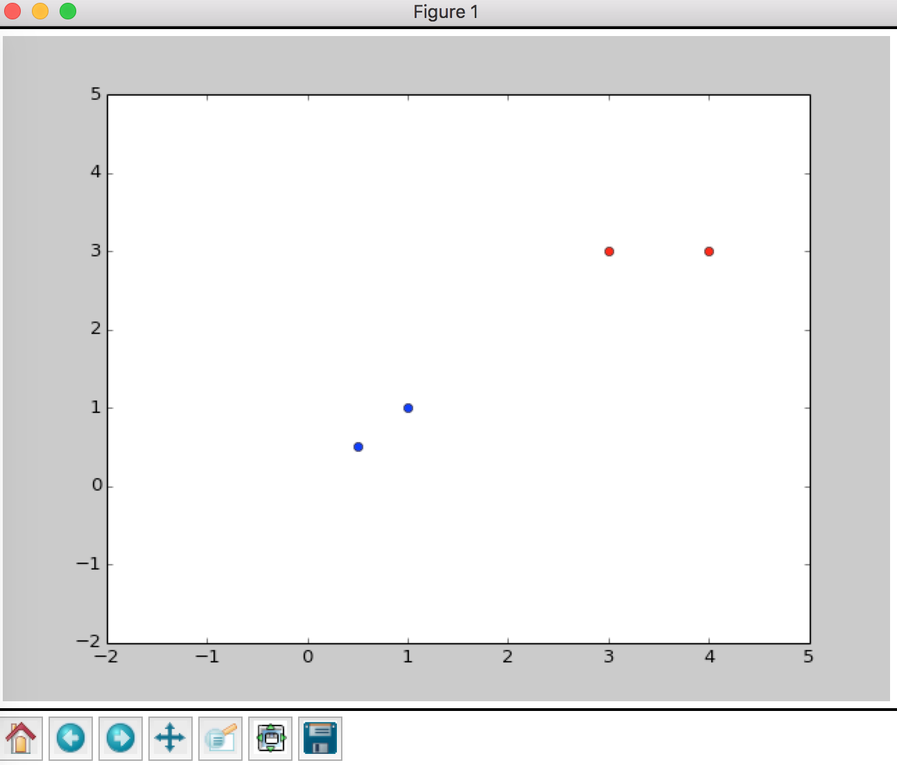
It's clear that the simple dataset is divided into two groups.

We need a function to decide whether we have classify all data correctly, if not, return a misclassified data.

def done(X, Y, W, b):
    for x, y in zip(X, Y):
        if (W.T.dot(x) + b) * y <= 0:
            return False, x,y
    return True,None,None

Do initialization

W = np.array([0,0],dtype=np.float64)
b = 0.0
datas = []

while True:
    _done, x,y = done(X,Y,W,b)
    if _done:
        break
    else:
        W += y*x
        b += y
        datas.append([W.copy(),b])
print 'parameters: ',W,b

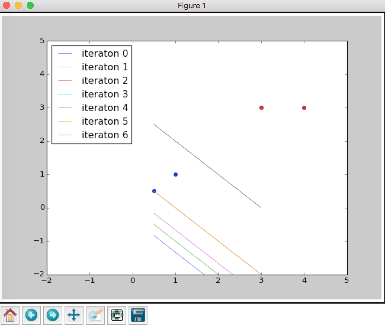
Updata $W$ and $b$ if dataset is not perfectly classified.

And plot the hyperplane after each iteration.

xs = np.array([np.min(X[:,1]), np.max(X[:,1])],dtype=np.float128)
for k,para in enumerate(datas):
    ys = -(para[0][0]*xs+para[1])/(para[0][1])
    plt.plot(xs,ys,label='iteraton {}'.format(k),lw='0.5')


plt.legend(loc='best')
plt.show()

The output is

parameters:  [1. 1.] -3.0

(Dual Problem)

In original problem, we set $w$ and $b$ to 0, and when there's a misclassified sample $(x^{(i)},y^{(i)})$, with updata $w$ and $b$ with the following rule

Suppose for each sample$(x^{(i)},y^{(i)})$, update parameters $n_i$ times

where

The output model is

Formally, the algorithm is

a_i = 0, b=0
while(there are misclassified sample){
    choose a misclassified sample;
    a_i := a_i + η
    b   := b + ηy_i
}

Since all samples only appear as inner product in dual problem, we can store a matrix with inner products, this matrix is called Gram Matrix.

Now let's implement the dual problem in python

(Dual problem implementation)

let's create another file. First, we need our silly dataset.

import numpy as np

def getDataSet():
    X = np.array([
        [3, 3],
        [4, 3],
        [1, 1],
        [0.5, 0.5]
    ], dtype=np.float64)


    Y = np.array([1,1,-1,-1], dtype=np.float64)
    return X,Y

The done() function is a lot different from the one in original problem. Here $a_i$ is a python dictionary stores how many times a sample is trained on, since np.ndarray is unhashable, we use index instead; and the $gram_mat$ is the Gram Matrix stores the inner product of samples.

The second for loop is the accumulated sum

def done(X, Y, a_i, b, gram_mat):
    for i in range(len(Y)):
        w_x = 0
        for j in range(len(Y)):
            w_x += a_i[j]*Y[j]*gram_mat[i][j]
        if Y[i]*(w_x+b)<=0:
            return False, i

    return True,None

And since we need to store a Gram Matrix, let code the perceptron as a class.

class Perceptron():
    def __init__(self,X):
        self.X = X
        self.gram = np.matmul(X, X.T)
        #self.W = np.zeros(shape=[2],dtype=np.float64)
        self.W = np.zeros(shape=[X.shape[1]], dtype=np.float64)
        self.b = 0.0
        self.a_i = dict()
        for i in range(len(X)):
            self.a_i[i] = 0

        print 'gram: ',self.gram

    def parameters(self):
        return self.W, self.b

    def train(self,Y):
        while True:
            _done,i = done(self.X, Y, self.a_i,self.b, self.gram)
            if _done:
                break
            else:
                self.a_i[i] += 1
                self.b += Y[i]

        for j in range(len(Y)):
            self.W += self.a_i[j]*Y[j]*self.X[j]


    def predict(self,inX):
        #pred = self.W[0]*inX[0] + self.W[1]*inX[1]+self.b
        pred = np.inner(self.W,inX) + self.b
        if pred > 0:
            return 1
        else:
            return -1


X,Y = getDataSet()
p = Perceptron(X)
p.train(Y)
print 'parameters: ',p.parameters()

The output is

gram:  [[18.  21.   6.   3. ]
 [21.  25.   7.   3.5]
 [ 6.   7.   2.   1. ]
 [ 3.   3.5  1.   0.5]]
parameters:  (array([1., 1.]), -3.0)

We got the same paramters one the same dataset, so the prediction and plot must be the same.