Naive Bayes

Basic Principle

Naive Bayes learn the prior distribution $P(Y)$and conditional distributon $P(X|Y)$from training dataset, and so learn the joint distribution$P(X,Y)$.

Strategy

Suppose we have a training dataset

Naive Bayes assume all $x's$ are independent, for formally

and that's why it's "Naive" Bayes. Actually the assumption is not so reasonable, for example, when doing spam email classification where $X_i∈\{0,1\}$, indicating whether a word exists in the email or not. $P(X_{Naive})$ and $P(X_{Bayes})$ may be correlated to some degree, because if there's word "Naive", it's more likely that there's word, so $P(X_{Naive}=1,X_{Bayes}=1)$ may be larger than $P(X_{Naive}=1)*P(X_{Bayes}=1)$.

Althrough the assumption is not so true, Naive Bayes algorithm is extremely effective.

Naive Bayes learns the conditional distribution $P(X|Y)$, more intuitively, how the example looks like given the label, or say, the machanism how a sample is generated, so it's actually a generative model.

Naive Bayes learn $P(Y)$ and $P(X|Y)$ directly from training data, and when doing prediction, we compute posterior distribution using Bayes Theorem.

When doing prediction, the strategy is

And the model training can be expressed as (on training set)

This leads to the joint likelihood form. On the whole training data, the joint likelihood is

Parameters (Maximize Likelihood Approximation)

To make the prediction better, we need some parameters to maximize the joint likelihood. Assume we have a training set of size $m$, and each $x$ has $a$ probabe values .

The log joint likelihood is

And the model training is

It should be very straight forward why these parameters maximize the likelihood, for the formal proof, check here.

Maybe you're wondering what the $+k$, $+a$, $+1$ terms. Now let's find out why.

Laplace Smoothing

When do the prediction

If for some $x_i$ have $P(x_i|y=k)=0$, then both the denominator and numerator are $0$ and. That's a trap, and so we need a "smooth". Take $φ_{y=k}$ as an example, it's unfair to say that $P(y=k)=0$, or say, $y$ can't be of label $k$ just because we haven't see $y=k$ in our finite training sample. Notice that it still holds true that

which is a desired property.

Algorithm

Suppose we have training set

where

and $x^{(i)}_j$ has $a_j$ possible value.

(1) Compute prior distribution $P(Y)$ and conditional distribution $P(X|Y)$

(2) For a given $x=(x_1,x_2,...,x_n)$, compute

Naive Bayes Variation: Multinomial Event Model

Take spam email classification as an example. In the Naive Bayes model above, suppose our considered 50000 words, then each training sample is

$x_j$ is whether the $j$th word appers or not, but actually, how often a word appears really matters. So in Multinomial Event Model, we take it in count.

Now $x$ is

$x_j$ is the index of the $j$th word in the vocabulary , and $n_i$ is total number of words in the $i$th sample, $|V|$ is how many words we take into consideration, or say, vocabulary capacity.

And the conditional distribution parameter $φ_j$ is how many the $j$th word appears in all spam email.

The numerator is how many times the $k$th number appears in all spam emails, and $+1$ is for Laplace Smoothing

And the prior distribution is pretty much the same.

Implementation (Naive Bayes)

Suppose we have some postings on a forum, the following number indicates whether the post is abusive. 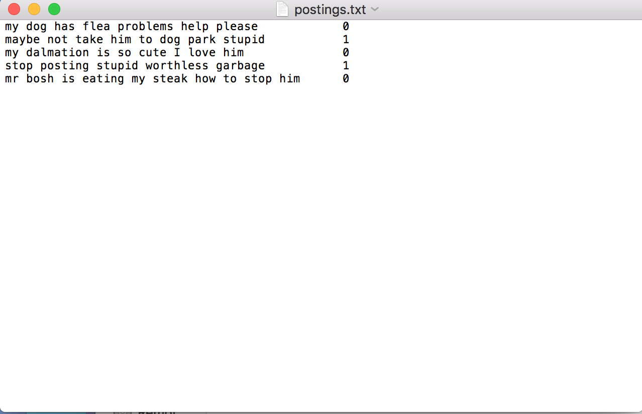There're only a few word, you can type them by hand.

First, we need to preprocess the data.

• Read the post and labels respectively.
• Generate the vocabulary list from the postings.
• Generate word list for each post.

import numpy as np

def loadDataSet(filename):
    postings = []
    labels = []
    for line in open(filename):
        words = line.split()
        posting = words[:-1]
        label = int(words[-1])
        postings.append(posting)
        labels.append(label)
    return postings, np.array(labels)

def createVocabularyList(dataset):
    wordsSet = set()
    for data in dataset:
        for word in data:
            wordsSet.add(word)
    return list(wordsSet)

def setOfWordsToVec(vocabularyList, dataset):
    ret = []
    for data in dataset:
        returnVec = [0]*len(vocabularyList)
        for word in data:
            if word in vocabularyList:
                returnVec[vocabularyList.index(word)] = 1
            else:
                print('word "{}" is not in the vocabulary list'.format(word))
        ret.append(returnVec)
    return np.array(ret)

In the function setOfWordToVec, for each sample data, the feature is of the same size as vocabularyList, the $i$th digit indicats whether the $i$th word in the vocabularyList appears in the sample data.

postings, labels = loadDataSet('postings.txt')
vocabularyList = createVocabularyList(postings)
vecs = setOfWordsToVec(vocabularyList, postings)

for vec in vecs:
    for i in range(len(vec)):
        if vec[i] == 1:
            print(vocabularyList[i],end=' ')
    print()

The output is

has flea problems help my dog please 
him maybe park not take dog to stupid 
him is so I cute dalmation love my 
worthless garbage stop posting stupid 
steak him is bosh how mr my eating to stop 

The words maybe in different order, that's because we use python dictionary in function createVocabularyList, but that's there words.

And now we need a function to fit the parameters (with Laplace Smoothing) according to the formulas. In this function, we use the processed word vectors, which words are in the fixed order, same order as in the vocabulary list.

In this function, we use the processed word vectors, which words are in the fixed order, same order as in the vocabulary list, or the probability of each word will be messed.

def trainNaiveBayes(trainSamples, trainLabels):
    num_train = len(trainSamples)
    numwords = len(trainSamples[0])

    
    # prior distribution φ_{y=1} = P(y=1)
    num_y_1 = len(np.flatnonzero(trainLabels))
    phi_y_1 = (float(num_y_1))/(num_train)
    phi_y_0 = 1. - phi_y_1


    # φ_{j|y=1} = P(x_j|y=1)
    # φ_{j|y=0} = P(x_j|y=0)
    samples_y_1 = trainSamples[trainLabels==1]
    samples_y_0 = trainSamples[trainLabels==0]

    # log scales phi_j in case underflow
    phi_j_y_1 = np.log(
        (np.sum(samples_y_1,axis=0) + 1)/(len(samples_y_1) + numwords)
    )
    phi_j_y_0 = np.log(
        (np.sum(samples_y_0,axis=0) + 1)/(len(samples_y_0) + numwords)
    )

    return {
            'phi_y_1':phi_y_1,
            'phi_y_0':phi_y_0,
            'phi_j_y_1':phi_j_y_1,
            'phi_j_y_0':phi_j_y_0
            }

Now we need to do prediction with the fitted Naive Bayes Model. Remeber the formula

Our strategy when doing prediction is

The demominator is a sum over $y$, so we just need

Instead use the formula directly, we compute log-likelihood. The formula is same as

Remeber we calculate $log$phi_j_y_1 in the function trainNaiveBayes, now we use the log term.

def classifyNaiveBayes(vecs,parameters):

    phi_y_1 = parameters['phi_y_1']
    phi_y_0 = parameters['phi_y_0']
    phi_j_y_1 = parameters['phi_j_y_1']
    phi_j_y_0 = parameters['phi_j_y_0']

    ret = []
    for vec in vecs:
        p_y_1 = np.sum(vec*phi_j_y_1) + np.log(phi_y_1)
        p_y_0 = np.sum(vec*phi_j_y_0) + np.log(phi_y_0)
        print('p_y_1:', p_y_1)
        print('p_y_0:', p_y_0)
        print()
        if p_y_1 > p_y_0:
            ret.append(1)
        else:
            ret.append(0)

    return np.array(ret)

Now we test how the Naive Bayes Model performs.

def loadTestingData():
    return[
        ['you','stupid','thing'],
        ['I','love','him'],
        ['he','is','a','stupid','garbage']
    ]

Clearly the first and third sentence is abusive.

postings, labels = loadDataSet('postings.txt')
vocabularyList = createVocabularyList(postings)
wordVecs = setOfWordsToVec(vocabularyList, postings)
state = trainNaiveBayes(wordVecs, labels)


testData = loadTestingData()
testVecs = setOfWordsToVec(vocabularyList, testData)
testLables = classifyNaiveBayes(testVecs, state)
print(testLables)

The output is

word "you" is not in the vocabulary list
word "thing" is not in the vocabulary list
word "he" is not in the vocabulary list
word "a" is not in the vocabulary list

p_y_1: -3.251665647691192
p_y_0: -3.9765615265657175

p_y_1: -10.525105164769647
p_y_0: -8.42312668237717

p_y_1: -9.426492876101538
p_y_0: -9.80942104349706

[1 0 1]

You can see that the Naive Model didn't show much confidence on the first and third sample, that's because our training data is small, for some words, the model doesn't "know" exactly whether it's abusive or not.

For Multinomial Event Model, you may check CS229 Assignment.