KL Divergence

In this note we'll learn KL Divergence, which is an important concept in Machine Learning. I'll use the example found at here, but there's something I'd like to share in detail.

Problem we try to solve

Think about it. A group of astronauts find a planet where lives space worms. Their teeth are their weapons. The astronauts risked their life and did some sampling on the teeth number of worms of a total number of 100. And the result is like

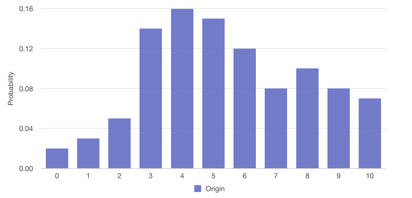
And to estimate the risk the astronauts will face, we want to fit the sample to a probability distribution, so that they can roughly know how scary a monster they'll meet.

First try, Uniform Distribution

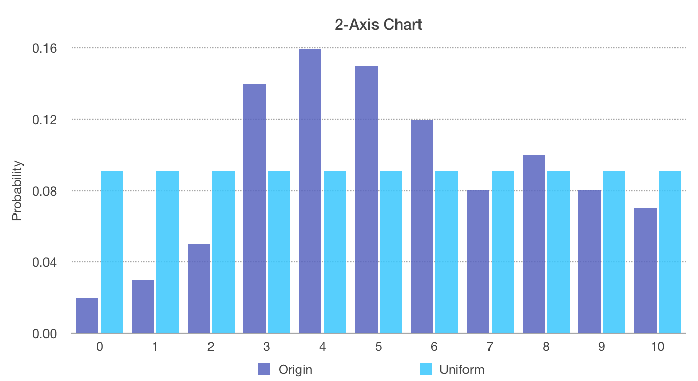
First, we try to fit this sampling to a Uniform Distribution.

Uniform Distribution has only one parameter, the probability of a given event happening.

p\_uniform = 1/total\_events = 1/11 = 0.0909

Put original and the uniform distribution we fit together

Second try, Binormial Distribution

In Binomial Distribution, we enumerate each possible tooth as "there is" and "there isn't". For each possible tooth, the pobability of "there is" is given by parameter $p_{binomial}=p$ , and the probability of "there is k teeth" is given by

C_n^k~p^k~(1-p)^{n-k}

where

C_n^k = \frac{P_n^k}{k!} = \frac{n(n-1)(n-2)...(n-k+1)}{k!} = \frac{n!}{k!(n-k)!}

The intuition is that first we pick k teeth from n positions, and for each of k existing teeth, the probability of "there is" is $p$ ; and otherwise the probability of "there isn't" is $1-p$ .

Additionally, for n example, the expected(mean) value of a binormial distribution is $expectation=np$ ,that is, if you toss a coin for $n$ times and each toss the probability of getting head is $p$ , if you do the experiment for $m$ times, $\frac{total~num~of~head~through~m~times}{m}$ will be $np$ , or say, for each expriment, it's expected to $np$ heads.

And the variance is $variance=np(1-p)$ . Suppose we toss a coin which follow a binomial distributionfor n times and probability we calculate of getting a head is $p$ . The variance is given by formula(suppose that head is 1 and tail is 0)

var = \frac{1}{n} \sum_{i=1}^{n}(x_i-mean)^2

= \frac{1}{n} \sum_{i=1}^{np}(1-p)^2 + \frac{1}{n} \sum_{i=1}^{n-np}(0-p)^2

= np(1-p)

And now back to modeling. For wach space worm, it's like a 11-time-toss(11 is the largest number of teeth), and each tooth of a space worm is a toss. So the expected value(mean) is

E = \sum^{n}_{i=1}p_ix_i

= 0.02*0 + 0.03*1 + 0.05*2 ... + 0.07*10

= 5.44

p_binomial = 5.44/10 = 0.544

So the probability of a 0-tooth worm is

p_0 = C_{10}^0~p^0~(1-p)^{10} = 0.0004

p_1 = C_{10}^1~p^1~(1-p)^{9} = 0.0046

p_2 = C_{10}^2~p^2~(1-p)^{8} = 0.0248

p_3 = C_{10}^3~p^3~(1-p)^{7} = 0.0792

p_4 = C_{10}^4~p^4~(1-p)^{6} = 0.1653

p_5 = C_{10}^5~p^5~(1-p)^{5} = 0.2367

p_6 = C_{10}^6~p^6~(1-p)^{4} = 0.2353

p_7 = C_{10}^7~p^7~(1-p)^{3} = 0.1604

p_8 = C_{10}^8~p^8~(1-p)^{2} = 0.0717

p_9 = C_{10}^9~p^9~(1-p)^{1} = 0.019

p_{10} = C_{10}^{10}~p^{10}~(1-p)^{0} = 0.0023

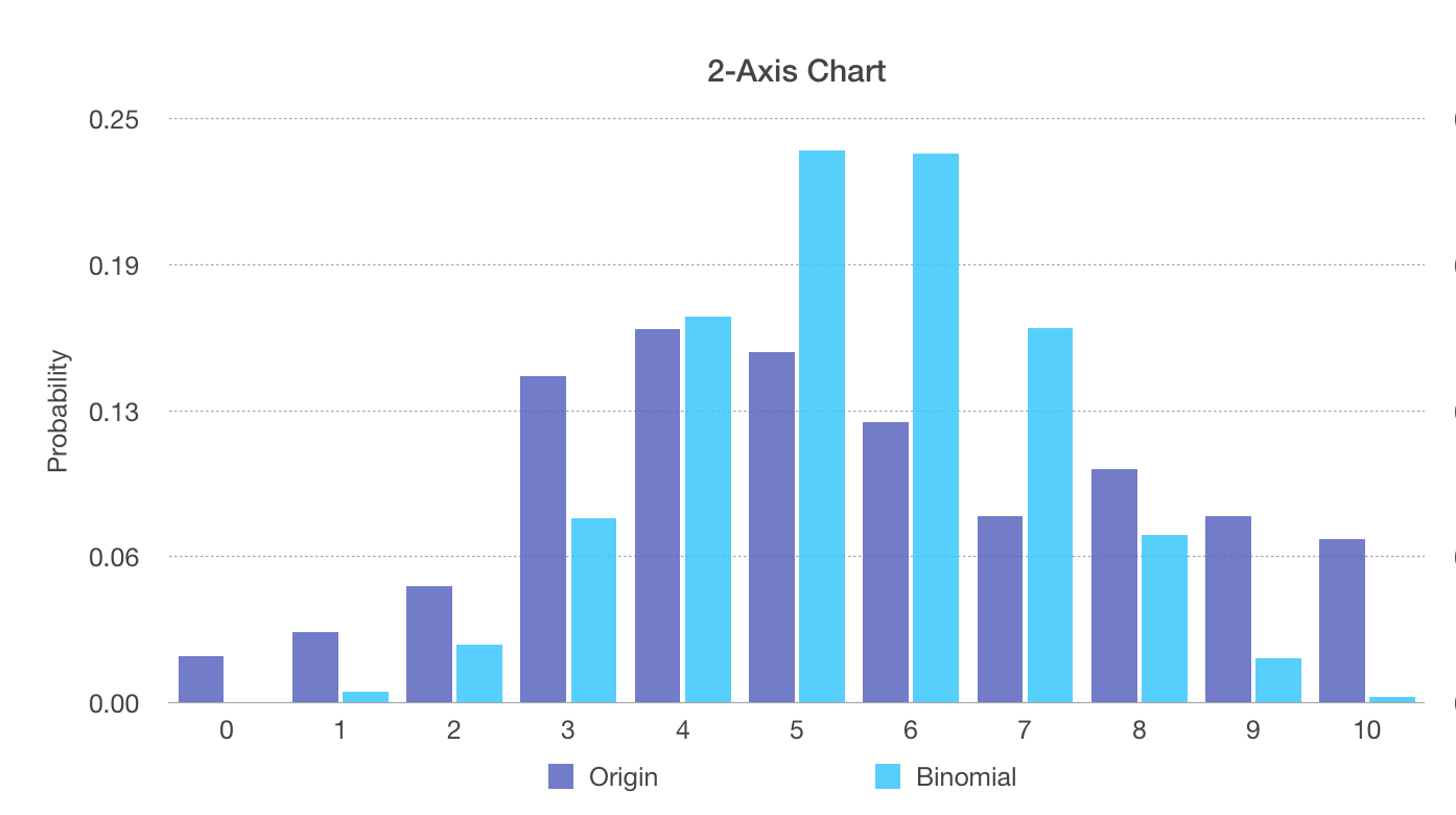
Put original distribution and binomial distribution together, it looks like

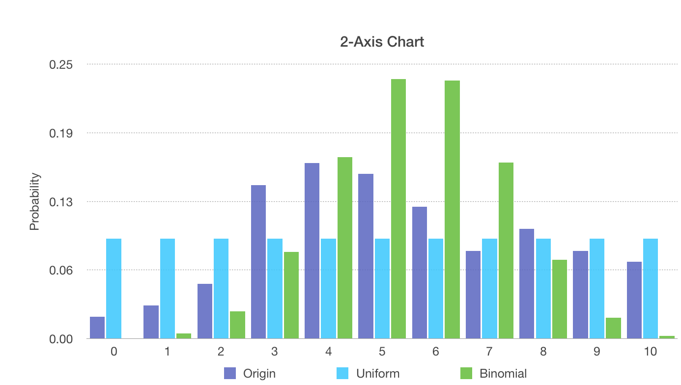
Put all these three distributions together.

KL Divergence

Now we fit the original probability distribution to 2 uniform distribution and binomial distribution, we want to pick the one with better fitting, but how to me measure which one is better? That's where KL Divergence comes in.

Let's assume the original distribution is $p(x)$ and the distribution we fit is $q(x)$ . The KL divergence is defined as

D_{KL}(p||q) = \sum_{i=1}^n p(x_i) log(\frac{p(x_i)}{q(x_i)})

The intuition is, $\frac{p(x_i)}{q(x_i)}$ indicates how much $p(x_i)$ differs from $q(x_i)$ , and $log$ maps the difference to a zero-based number, the closer $q(x_i)$ is to $p(x_i)$ , the less the $log$ term is; when $p(x_i)=q(x_i)$ , the $log$ term is 0. And the $p(x_i)$ before the $log$ terms shows how much the difference at $x_i$ matters to the whole distribution, if $p(x_i)$ is almost $0$ , it doesn't matter much even if $p(x_i)$ differs a lot from $q(x_i)$ .

And now, back to our two distributions, which one is a better fit?

First let calculate $D_{KL}(original||uniform)$ with python.

import numpy as np

uniform = []
for i in range(11):
    uniform.append(0.0909)
uniform = np.array(uniform)

binomial = np.array([
    0.0004,
    0.0046,
    0.0248,
    0.0792,
    0.1653,
    0.2367,
    0.2353,
    0.1604,
    0.0717,
    0.019,
    0.0023
])

real = np.array([
    0.02,
    0.03,
    0.05,
    0.14,
    0.16,
    0.15,
    0.12,
    0.08,
    0.1,
    0.08,
    0.07
])

Now we need a function to calculate KL divergence from two distributions. Remeber the formula is

D_{KL}(p||q) = \sum_{i=1}^{n} p(x_i)log(\frac{p(x_i)}{q(x_i)})

def KL_Divergence(dis1, dis2):
    ret = 0.0
    for i in range(len(dis1)):
        ret += dis1[i] * np.log(dis1[i]/dis2[i])

    return ret
    
DL_real_uniform = KL_Divergence(real, uniform)
DL_real_binomial = KL_Divergence(real, binomial)

print "KL(real||uniform): ", DL_real_uniform
print "KL(real||binomial): ", DL_real_binomial

The output is

KL(real||uniform):  0.13677971595000277
KL(real||binomial):  0.42657918710043913

Actually, the uniform distribution is a better fit.